
Flow stability
This page is a not-really-orthodox introduction to the concept of flow instabilities, especially applied to boundary layers, with some references to the receptivity mechanism and to flow control. If you are already familiar with these topics, you should start navigating the menu on the left. If you are not, I would strongly recommend to keep reading.
TopA romantic introduction to flow stability
Every-day life experiences contain some simple insights for the understand of flow stability. Have you ever seen the smoke from a cigarette? If not, look at the picture below, which is a marvelous flow visualization of one of the most important, and not-yet-understood, physical phenomenon. Unfortunately I was not able to find a nice picture of the smoke from a chimney or the water from a tap as good as this one, otherwise I would have used an example different from smoking. Smoking is dangerous, so please do not smoke!
Figure 2. Smoke from a cigarette. Please, do not smoke!
The smoke is just a trick to visualize what happens inside the air. When the fluid is regularly moving, the flow regime is called laminar, when it shows very complicated and strange patterns it is called turbulent and the route from the former to the latter is called transition for obvious reasons. The laminar flow regime is characterized by order, predictability, low mixing and almost absent diffusion. The smoke just at the end of the burning cigarette behaves in this way, as clearly shown in the picture. The turbulent flow regime is exactly the opposite. It features high disorder, random unsteadiness, apparent unpredictability, very high mixing and diffusion. The region in the picture labeled as "Turbulence" should give an idea of what this means.
Laminar flows, in nature, experience a fatal poor resistance that make them become turbulent. For this reason it is quite difficult to find example of laminar flow in every-day life, while it is much simpler to enumerate turbulent flows such as the coffee mixed in a cup so as to make it cool down, the water coming out from any tap, the smoke rising from a chimney, any river worthy of its name.
TopThe concept of stability applied to a boundary-layer flow
What is a boundary layer? Every time a body interacts with a fluid, a thin layer arises in the vicinity of the body surface. At the interface between the fluid and the body, the velocity of the fluid is zero, because of the inter-molecular-force interactions. However, the velocity far from the body is non-zero (it has to reach the value of the oncoming flow) so that there exists a region, named boundary layer, in which the velocity field gradually varies from zero to the so called free-stream value. The boundary layer characterizes many of our every-day activities, from that originated by a small spoon used to mix the coffee, to a vehicle moving in air or water (bicycles, cars, trains, airplains, ships, submarines, etc.). We actually "live" in the boundary layer due to the atmospheric winds interacting with the earth surface!
The boundary layer on a body can be laminar or turbulent, exactly as the flow originating from the cigarette. If the flow is evolving in space (or time), the first region is laminar (the nose of an airplane fuselage or the leading edge of the wing) whereas after a certain location it becomes turbulent. The explanation of why, when and where the transition from laminar to turbulent flow occurs is related to the concept of stability.
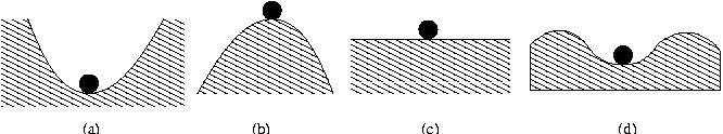
Figure 3. (a) stability, (b) instability, (c) neutral stability, (d) stability to small perturbation.
A simple and effective example of what stability means is reported in the above figure. If the ball in figure 3 case (a) is moved from its original position, it always comes back where it was. On the contrary, the ball in figure 3 case (b) continuously moves away and does not come back to its original state when touched, even very slightly. Case (c) in figure 3 is particular since it is insensitive to any perturbation. Finally, the ball in figure 3 case (d) comes back to the original state only if the perturbation is weak. If it is strong enough to make the ball overcome the two bumps, however, the original position is no more reached.
Bearing this example in mind, a physical system is defined stable if, after a disturbance has been applied, it returns to its original state (case (a)), unstable if it never returns back to the original state (case (b)), neutrally stable if the system is not sensitive to any perturbation (case (c)) and stable for small disturbances if it returns to the original state only if the perturbation applied is small, whereas it never returns if the perturbation is larger than a certain threshold (case (d)). It should be clear also that the stability is always referred to a certain original state, called basic state.
How does all this apply to fluid mechanics? In fluid dynamics the basic state is called basic flow and it is usually laminar (for instance, the air on a wing or car surface, the water on a submarine surface, etc.). The laminar flow can be stable or stable for small disturbances if it returns to its original state respectively after any disturbance or a small disturbance has been applied. On the contrary, the laminar flow is unstable if any disturbance does not die out but grows changing the laminar state to another. This other state is usually and commonly the turbulent flow but it could be also a more complicated laminar one.
At this point, the example of the cigarette , should look like a good visualization of stability applied to fluid mechanics. The original state (the laminar flow just at the end of the cigarette) undergoes an instability process that leads to the turbulent flow state. This particular laminar flow is thus unstable. Looking at the cigarette, it should be clear what the effect of a fluid dynamic instability is.
Under which conditions does the flow become unstable? The answer to this question is still open and it is the object of fluid-dynamic instabilities study. A common feature, however, seems to be the dependence on a parameter called Reynolds number, which represents the relative importance of the convective and inertial mechanisms to the dissipative ones. Experiments show that in very high Reynolds-number flows, turbulence eventually develops. The first experimental evidence of this dependence was demonstrated by Reynolds in his famous pipe-flow experiences. He noticed that transition from laminar to turbulent flow can occur if Re is larger than a certain characteristic value called critical Reynolds number Recr. Without entering the details, we remark that Recr is the value of the Reynolds number for which the laminar flow shows the beginning of the instability process. This does not necessarily mean that the flow will develop towards turbulence, since damping effects could avoid that. However, if the flow becomes turbulent, Retr is the transitional Reynolds number, defined as the value at which the flow is already fully turbulent.
TopFlow Receptivity
Now that we know what a fluid dynamic instability is, the next natural question one should ask is: how is a fluid dynamic instability excited? It is clear that the ball in figure 3 case (b) is unstable. However, if it is not moved, it can stay in equilibrium for ever! On the other hand, if an external exciting source is applied to the ball, the instability actually takes place. The ball, moved from the equilibrium position, does not return to its original state anymore. It is thus clear that first an exciting disturbance is needed, secondly an exciting mechanism should introduce the exciting source into the system.
Reynolds, in his experiments (1883), had to deal with the problem of the external disturbances and how they influence the flow. He found a strong dependence of the onset-transition spatial location on the environmental conditions. He used a tank full of water connected to a pipe and put a needle at the beginning of the tube in order to let a dye filament visualize the flow pattern. He noticed that if attention was paid to the design of the connection between the reservoir and the pipe, transition could be delayed. If the pipe-fitting was too sharp or if roughness was present inside the duct, however, transition was anticipated. Moreover, the same experiments have been recently repeated in a city laboratory, finding critical Reynolds numbers lower than those reported by Reynolds himself, probably because of the vibrations induced by cars, trams, undergrounds, trains, etc., not present in Reynolds' laboratory. All these experiences show how much transition is related to the external environment in which exciting sources can be identified.
Transition, however, cannot occur if the exciting source is not introduced into the flow. The way by which the external disturbances can enter inside a particular flow is nowadays called receptivity. Obviously, receptivity does not necessarily mean instability or transition. If the basic flow is stable or if the perturbation is too weak to lead to the onset of the instability, or if damping effects arise, the flow continue behaving in a laminar regime. If the flow turns out to be unstable, the instability develops and eventually leads the flow to the turbulent regime. An important feature of the receptivity mechanism is that it relates the external disturbances to the stability properties of the flow under investigation. This allows us to predict transition as a function of the environmental conditions. Coming back to the introductory example, if the cigarette is slightly touched or some air blows on the final part of the cigarette (i.e. environmental disturbances are applied), then the laminar behavior is much shorter in space or even absent. The reason resides in the receptivity mechanism, which makes the external perturbations enter the flow and interfere with its stability characteristics.
TopFlow Control
The smoke from the cigarette eventually becomes turbulent anyway, spreading around and showing that turbulence is characterized by three-dimensionality and large diffusion. These features imply an increase of the mixing, so that turbulence can be welcome or unwelcome depending on the practical application for which it is studied.
Every time high mixing is required, turbulence is desirable. Chemical reactions represent the typical case where high exchange allows the species to get in touch very fast and accelerate the process. Another extremely important process driven by turbulence is the dilution of polluting dispersions. Life in cities is possible only thanks to the mixing of fresh air to the smog. Moreover, turbulence implies very high heat transfer rates and therefore it is welcome in heating or cooling processes (that is why we usually blow on hot coffee, tea or soup!).
On the contrary, the high mixing rates of turbulent flows are usually unwelcome in aerodynamic or hydrodynamic fields such as design of turbines, low-velocity vehicles, submarines, subsonic and supersonic civil and military aircrafts, hypersonic and reentry vehicles. The main problems related to latter applications are the increase of drag and heat loads. In fact, every object moving in a fluid experiences drag due to viscous effects (boundary layer). Turbulent drag, however, is greater than the laminar one, implying a much greater amount of fuel or energy needed in order to move through the fluid. On the other hand, significant heat loads due to turbulence introduce structural difficulties in supersonic or hypersonic applications.
Probably everyone who works with turbulence or laminar-to-turbulent transition would like to control flow instabilities and their consequences related to turbulence. The traditional view of turbulence (at least for the last 70 years) has been that it "forgets" its origins, and evolves towards a state that is independent of its upstream or initial conditions. This would mean that nothing can be done in the upstream region in order to affect what ultimately happens downstream. In other words, no control would be possible, other than local active control.
New ideas have been spreading over the past decade or so, suggesting that turbulence does not forget where it comes from. From a fundamental and practical point of view, this is quite exciting because it implies that we can influence turbulence by the way it is generated. Therefore, transition becomes very interesting as a means of turbulence control.
Learning how to control turbulence, or at least partially control it, can lead to huge benefits, such as reduced energy consumption as well as less noise and other environmental effects in water and air. It has been estimated that if laminar flow could be maintained on the wings of a large transport aircraft, a fuel saving of up to 25% would be obtained.
Flow control can have, in general, different purposes. In aeronautical applications drag reduction and therefore laminar flow control (LFC) is the main goal. In certain cases, however, such as the flow on the fuselage, a laminar flow cannot last because sooner or later the Reynolds number exceeds the transitional one. Other solutions are thus seek, as turbulence control and drag reduction.
As far as LFC is concerned, different strategies are possible. The laminar flow can be maintained avoiding transition to turbulence or the turbulent flow can be obliged to become laminar again (relaminarization). In any case, control techniques are applied. Different possibilities include shaping the body such that the flow is laminar as long as possible, looking for the best "aerodynamic shape". Another possibility is to delay transition acting on the basic flow and changing its stability characteristics, for example applying boundary layer suction or blowing at the wall. The power usually required in order to suck or blow, however, is much greater than the gain in drag reduction, making this approach quite useless.
As far as turbulence drag reduction is concerned, micro-grooves (riblets or similar) produced over otherwise smooth surface of the object, such as aircrafts, ships or automobiles can provide turbulent drag reduction of up to 10%. This passive device is believed to modify the structure of the turbulent boundary layer in such a way as to reduce the turbulent energy production, hence the drag reduction.
All the techniques outlined above are known as passive control. This means that the control has been decided a priori and cannot adapt itself to new situations or changes in the flow field. More sophisticated techniques "feel" the flow field and change some wall quantities in order to control the flow around the solid body. The great benefit, in this case, is that if the conditions change and are different from the "design" ones, the control can be still effective. For obvious reasons, this is called active control.
For more details on each of the aforementioned issue, browse the menu on the left.
Top