You should read this document before
performing the Christmas Assignment.
Here, you can find already-solved-exercises
as a training for the Christmas Assignment.
We will resort on and establish the standard
procedures and approaches to derive the solutions.
We will also propose the use of the tableau
as a convenient way to store and represent dictionaries.
The use of the tableau
as an handy and compact notation for dictionaries
is also the most common standard when teaching LP.
Offen,
the several theoric and algorithmic aspects
of LP are introduced as methods for manipulating and inspecting the
tableau entries
to get the desired results or seek the answers to the pertinent questions.
If you will meet LP again in the future,
it is quite likely that you will have to resort on the skill of knowing how to
read a tableau.
For this reason, it is a good idea to
adopt this approach right now
and achieve fluency in its language and mastery
in its technicality.
When performing the Christmas assignment,
we recommend you to make use of the tableau
since representing all steps in a compact form increases
clarity and readability.
As a matter of fact,
the tableau offers the standard instrument
to increase the quality of the document produced
when solving LP problems.
Have a nice reading.
The tableau and the Simplex Method
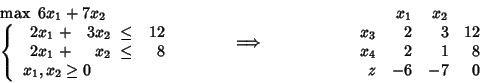
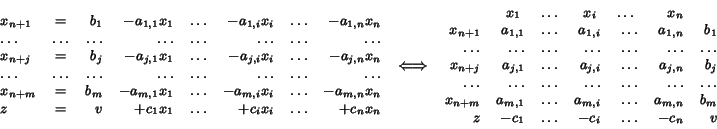
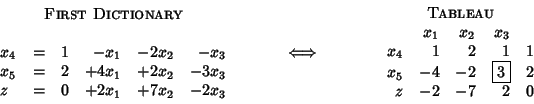
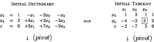
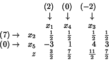
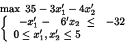
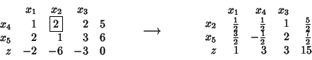
To the following LP problem we associate the corresponding tableau:
Where ![]() and
and ![]() are the names for the slack variables.
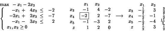
Note that the coefficients of the objective function
are put in the tableau with opposite signs
and that the objective function corresponds (in the most widespread
practice)
to the last row.
are the names for the slack variables.
Note that the coefficients of the objective function
are put in the tableau with opposite signs
and that the objective function corresponds (in the most widespread
practice)
to the last row.
To say it full, the tableau does not really correspond to an LP problem but to a particular dictionary of the problem, that is, to an LP problem as seen from the perspective of a basic solution (feasible or not). Here above, we have just ben lucky: since the problem was in standard form, it was very easy to fill in the corresponding tableau. Moreover, since the constant term in each constraint was non-negative, then the basic solution corresponding to this first tableau is feasible.
On the current solution,
the objective function assumes a specific numerical value,
which is reported on the right in the last row of the tableau.
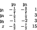
In general, the following dictionary is more compactly described as a tableau:
Here is a second example:
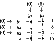
To choose the pivot row,
consider those
![]() which are positive.
Among these, that one which minimizes the ratio
which are positive.
Among these, that one which minimizes the ratio
![]() ,
is the pivot element.
,
is the pivot element.
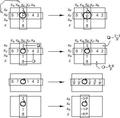
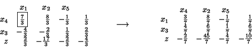
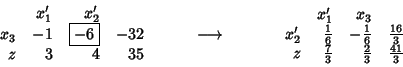
Let us pivot in the dictionary and observe what is pivoting in the tableau.
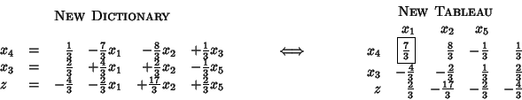
In the tableau,
let ![]() be the pivot row
and
be the pivot row
and ![]() the pivot column.
Let
the pivot column.
Let
![]() be the value of the pivot
element.
Here is the general rule to execute the pivot
directly on the tableau:
be the value of the pivot
element.
Here is the general rule to execute the pivot
directly on the tableau:
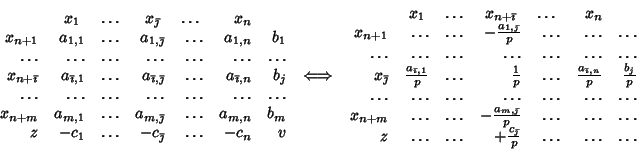
In conclusion, pivoting work as follows.
The pivot operation is illustrated in Figure 1.
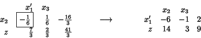
To practice, let us get back to our LP problem and let us perform the next pivot.
The elements in the last row
are now all negative.
We can therefore conclude that the optimal value
of our problem was ![]() .
(Why?)
The optimal primal solution is
.
(Why?)
The optimal primal solution is
![]() with
with
![]() and
and
![]() .
The optimal dual solution is
.
The optimal dual solution is ![]() with
with
![]() ,
,
![]() and
and
![]() .
Note that also the dual solution is expressed in the tableau.
.
Note that also the dual solution is expressed in the tableau.
As a matter of fact, we can even obtain the tableau for the dual from the tableau of the primal.
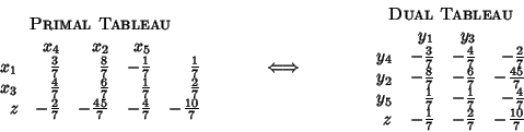
Where the dual decision variable ![]() corresponds to the primal slack variable
corresponds to the primal slack variable ![]() and is therefore
the multiplier of the first primal constraint.
The dual variable
and is therefore
the multiplier of the first primal constraint.
The dual variable ![]() corresponds to the primal variable
corresponds to the primal variable
![]() which is the multiplier of the first dual constraint;
therefore
which is the multiplier of the first dual constraint;
therefore ![]() is the surplus variable in the first dual constraint.
is the surplus variable in the first dual constraint.
When we are asked to maximize the objective function,
then we follow the same procedure,
with the only difference that now our aim is to make the elements
of the last row non-negative.
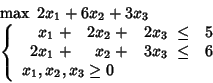
For example:
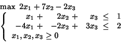
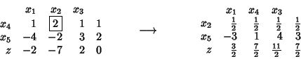
The optimal value of the objective function is now ![]() .
The optimal primal solution is
.
The optimal primal solution is ![]() with
with
![]() .
The optimal dual solution is
.
The optimal dual solution is
![]() with
with
![]() .
.
|
AN HANDY CHECK Even with LP we have our check of the nine to make sure that computations did not introduce any mistake until now. Just assign to each variable the value of the coefficient of the same variable in the original objective function. For example, the last tableau becomes:
For each column the following holds:
the value of the coefficient associated to the column
plus the value of the last element of the column
equals the sum of the other elements of the column each multiplied
by the coefficient of the row to which it belongs.
Column 1:
These relations hold for every tableau, not necessarily optimal.
|
The tableau and the Dual Simplex Method
Consider an LP maximization problem in standard form. Let us assume that all coefficients in the objective function are non-positive. Therefore, in the last row of the first tableau all coefficients are non-negative, precisely like we would like them to be in the last tableau. Such a tableau is called dual-feasible. If all coefficinets in the last column are non-negative, then the current basic solution is feasible and the problem is already solved. Otherwise we better apply the Dual Simplex Method. An interesting characteristic of the Dual Simplex Method is that the pivot operation is exactly the same as for the (Primal) Simplex Method. The only difference among the two methods is in the choice of the pivot element. As a matter of fact, while the actaul rule is different, the philosophy behind the rule is the same.
The choice of the pivot column is dictated
by the necessity of mantaining dual feasibility,
which will be the invariant for the Dual Simplex Method,
like primal feasibility was the invariant for the (Primal) Simplex Method.
Therefore, to choose the pivot column
we consider all the negative
![]() .
Among these,
that one that minimizes the ratio
.
Among these,
that one that minimizes the ratio
![]() ,
is the pivot element.
,
is the pivot element.
Here is an example:
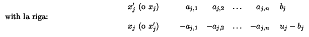
How to deal with bounds on the single variables
If instead of having ![]() , we have
, we have ![]() with
with ![]() , then we rely on the substitution:
, then we rely on the substitution:
![]() .
If a variable if bounded from above instead that
from below,
namely
.
If a variable if bounded from above instead that
from below,
namely ![]() ,
but
,
but ![]() is not required,
then we substitute
is not required,
then we substitute
![]() .
.
When however a non-negative variable is bounded from above,
such condition could be in principle regarded as a linear constraint
of the problem.
Nevertheless, when all variables are bounded
(and in most cases an obvious bound can be produced),
then we can take advantage of this special structure
by considering both the variable ![]() and the variable
and the variable
![]() and deciding to adopt in the writing of the first tableau the one of the two
which leads to a dual feasible tableau.
We then start with the Dual Simplex Method.
We must obviously guarantee that
and deciding to adopt in the writing of the first tableau the one of the two
which leads to a dual feasible tableau.
We then start with the Dual Simplex Method.
We must obviously guarantee that
![]() .
Moreover, through the various phases of the Dual Simplex Method
the dual feasibility is kept as an invariant,
and if one of the primal variables employed to express the tableau
(
.
Moreover, through the various phases of the Dual Simplex Method
the dual feasibility is kept as an invariant,
and if one of the primal variables employed to express the tableau
(![]() or
or ![]() ) becomes negative,
then a pivot step is executed
with the effect to get closer to primal feasibility.
It can happen however that a basic variable for the tableau
exceeds its own bound from above.
When this happens,
we replace the corresponding row in the tableau as follows:
) becomes negative,
then a pivot step is executed
with the effect to get closer to primal feasibility.
It can happen however that a basic variable for the tableau
exceeds its own bound from above.
When this happens,
we replace the corresponding row in the tableau as follows:
and then we can continue. For example:
After introducing the variables
![]() ed
ed
![]() ,
we choose to employ in the tableau the variables
,
we choose to employ in the tableau the variables
![]() and
and ![]() since the coefficients
of the objective function were both positive (and so?).
since the coefficients
of the objective function were both positive (and so?).
The sequence of tableax is therefore:
Now
![]() and therefore
the first row of the tableau is substituted introducing
and therefore
the first row of the tableau is substituted introducing ![]() :
:
Optimal solution: ![]() ed
ed ![]() with objective function
with objective function ![]() .
.
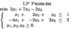
Sensitivity Analysis
Assume we are maximizing an objective function
which represents a profit or some other form of benefit.
The constraints will model limitations
in raw materials, goods or availabilities.
Then, the optimal values of the dual variables
will express the maximum ``price''
that we could pay to increment one unit of the availability
to which the dual variable is associated.
(From here the name ``shadow price'' or ``marginal value'').
We must however remember that the meaning of a shadow
price is strictly local: in generale
it will not be convenient to keep paying extra-units
of availability on the basis of the shadow price
for an arbitrary increase in availability.
Hence the question:
until when is the shadow price meaningful?
In other words,
what is the maximum increase in a certain facility
which we can pursue while paying for it the shadow price?
The answer can be easily obtained
with reference to the dual tableau.
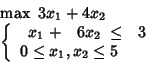
Assume for example that our target is to maximize the following profit:
where ![]() and
and ![]() express non-negative levels of activity,
whereas the constant terms in the constraints
express bounds on specific availabilities.
The tableau associated to the basic optimal solution is the following.
express non-negative levels of activity,
whereas the constant terms in the constraints
express bounds on specific availabilities.
The tableau associated to the basic optimal solution is the following.
Therefore we can consider paying (certainly not more than)
![]() for increasing by one unit the availability on the first
constraint.
But how much of this availability can we buy
at the price of
for increasing by one unit the availability on the first
constraint.
But how much of this availability can we buy
at the price of ![]() for each extra-unit?
Consider the dual of the last tableau:
for each extra-unit?
Consider the dual of the last tableau:
Assume we increment by ![]() the availability on the first constraint.
The advantage in considering the dual is that
the only row which is affected by this change
is the last one (corresponding to the last column in the primal tableau).
The next row can be produced by substitution
or we can make use of the HANDY CHECK seen above.
the availability on the first constraint.
The advantage in considering the dual is that
the only row which is affected by this change
is the last one (corresponding to the last column in the primal tableau).
The next row can be produced by substitution
or we can make use of the HANDY CHECK seen above.
Remember that for each column the following holds:
the value of the last element of the column
is obtained by summing up the other elements of the column, each multiplied
by the coefficient of the row to which it belongs,
and subtracting the value of the coefficient associated to the column.
Column 1:
![]()
Column 2:
![]()
Column 3:
![]()
Therefore, the last row is:
We can now easily discover that the tableau remains optimal
as long ad ![]() does not exceed
does not exceed ![]() .
We conclude that
.
We conclude that ![]() is the maximum increment in availability
for the first constraint that we are willing to buy
by paying
is the maximum increment in availability
for the first constraint that we are willing to buy
by paying ![]() for each extra unit.
If we are interested in determining
the price that we should be considering to pay for bigger increments
(the new shadow prices),
then we must execute a new pivot.
for each extra unit.
If we are interested in determining
the price that we should be considering to pay for bigger increments
(the new shadow prices),
then we must execute a new pivot.
| 2001-12-19 |
© Dipartimento di Matematica - Università di Trento
|